PrecisionCalc
xl Precision
Get Your Numbers Right

Format Negative Numbers
with Red Font

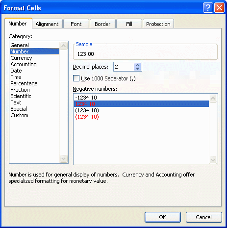
Normally, Excel allows you to format negative numbers with a red font:

However, that doesn't work with xlPrecision numbers, because Excel doesn't recognize them as numbers (and you wouldn't want it to, because then Excel would reduce the precision to 15 significant digits). But you can still get xlPrecision negative numbers to display with a red font, using Excel's Conditional Formatting feature.

It's easiest if you format xlPrecision negative numbers with parentheses and you're using Excel 2007 or later:

• Select the range of cells.
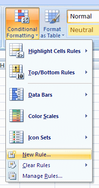
• Select: Home tab | Styles section | Conditional Formatting | New Rule
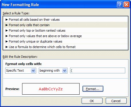
  • Select rule type: Format only cells that contain
  • Edit the rule description: Specific Text | beginning with | (
    • In the edit box, just type in an open parenthesis ("("), and nothing else.
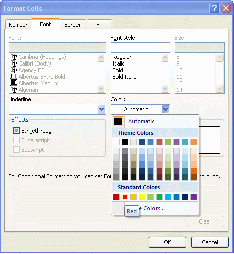
  • Click Format, change font color to red, and click OK.
  • Click OK.

If you format negative xlPrecision numbers with a leading hyphen ("-"), or if you're using Excel 2003 or earlier, you can still format negative xlPrecision numbers with a red font, but it's a bit trickier:

• Select the range of cells.
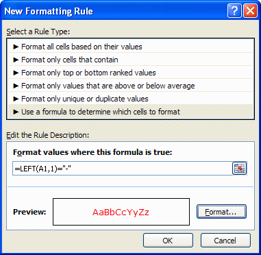
• Select: Formula Is
• Enter the formula:
  • Important note: the cell reference in the formula below must refer to the active cell in the selected range. So if you've selected column A, and cell A1 is the active cell, then the formula must refer to cell A1; then your conditional formatting rule will work for the entire selection, such as all of column A:
  • =LEFT(A1,1)="-"
    • In the formula above, be sure to replace "A1" with whatever cell is currently the active cell in the selected range.
  • Click Format, change font color to red, and click OK.
  • Click OK.
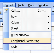
  • To get a red font for both parentheses and leading hyphens, you'll need two rules. To get the second rule in Excel 2007 and later, select Home tab | Styles section | Conditional Formatting | New Rule a second time and repeat the steps for the second rule.

In Excel 2003 and earlier:

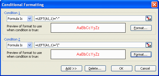
To get two rules In Excel 2003 and earlier, click Add to get "Condition 2" and repeat the steps for Condition 2:

xlPrecision Home Page
PrecisionCalc Home Page